Modelling, Simulation and Control of Hydro-Power System - Part 4
Implementing the model of lakes using DAE approach with Python
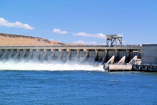 Image by Russ McElroy from Pixabay
Modular simulation of the lakes - Differential algebraic equation (DAE) conceptualization
This post shows one (of many) ways of implementing the nonlinear dynamics of a reservoir with non-linear outlet.
# imports
import numpy as np
import matplotlib.pyplot as plt
from scipy.optimize import minimize
Analytical solution to check correctness of implementation
To make sure that the results obtained by the numerical model reflects the correct dynamics of the lake, it is possible to compare it with analytical results of simple test cases. The reason not to always use these exact solutions is that it is not possible or trivial to obtain them in most real-world cases, therefore requiring a numerical model.
Draining reservoir, constant cross-section and non-linear outflow
The general formulation of the mass balance for the lake is:
$$ \frac{dm}{dt} = m_{in} - m_{out} $$
Where $m$ is the mass (of water) in the reservoir, $m_{in}$ is the mass flowrate entering the reservoir and $m_{out}$ is the rate of mass leaving the reservoir.
Rewriting $m = \rho Ah$, $m_{in} = \rho q_{in}$ and $m_{out} = \rho q_{out}$
$$ \frac{d(\rho A h)}{dt} = \rho q_{in} - \rho q_{out} $$
without loss of generality.
For the simplified case, let’s assume that:
- The reservoir has constant cross section $A$ ($A \neq A(t)$ and $A \neq A(h)$)
- The simulation involves only liquid (water), therefore the density $\rho$ can be considered constant ($\rho \neq \rho(t)$ and $\rho \neq \rho(P, T, V)$).
With these simplifications:
$$ \rho A\frac{dh}{dt} = \rho q_{in} - \rho q_{out} $$
$$ A\frac{dh}{dt} = q_{in} - q_{out} $$
For the simplified case, there is no inflow:
$$ q_{in}(t) = 0 $$
The outflow behaves as a free release. Using the steady mechanical energy conservation:
$$ c\frac{v^2}{2g} = h $$
Where $c$ is a correction factor, $v$ is the fluid velocity and $g$ is gravity acceleration ($\approx 9.81 m/s^2$).
Thus,
$$ v = c\sqrt{2gh} $$
$$ q_{out} = A_{orifice}v = A_{orifice}c\sqrt{2gh} $$
$$ A\frac{dh}{dt} = - A_{orifice}c\sqrt{2gh} $$
It can be rewritte and solved using separation of variables:
$$ A\frac{dh}{\sqrt{h}} = - A_{orifice}c\sqrt{2g} dt $$
$$ A \int_{h_0}^{h} h^{-\frac{1}{2}} dh = - A_{orifice}c\sqrt{2g} \int_{t_0}^{t} dt $$
The final solution is:
$$ 2A (\sqrt{h} - \sqrt{h_0}) = - A_{orifice}c\sqrt{2g} (t - t_0) $$
Let’s now use some values to obtain values of height of water at different points in time.
I’ll take the values used by Himmelblau (2006) in Example 32.2, which in summary says:
“A tank with cross section 16 $m^2$ and 10 meters height is full of water. Find the time required to empty the tank through an oriffice at the bottom of 5 $cm^2$. Use $c=0.62$”
Translating the values given to the solution obtained above:
- $A = 16$
- $h = 0.0$
- $h_0 = 10$
- $A_{orifice} = 5 \cdot 10^{-4}$
- $t = ??$
- $t_0 = 0$
- $c=0.62$
$$ 2A (\sqrt{h} - \sqrt{h_0}) = - A_{orifice}c\sqrt{2g} (t - t_0) $$
$$ 32 \sqrt{10} = 5 \cdot 10^{-4} 0.62 \sqrt{19.62} t $$
$$ t = \frac{32 \sqrt{10} }{5 \cdot 10^{-4} 0.62 \sqrt{19.62}} $$
$$ t \approx 7.37 \cdot 10^4 s \approx 20h 28 min $$
That’s the time required to empty the reservoir.
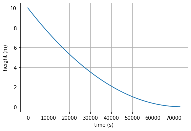
We can additionally implement a small piece of code to calculate the height at different points in time, making the final height as unknown:
$$ h = (- \frac{A_{orifice}c\sqrt{2g} (t - t_0)}{2A} + \sqrt{h_0})^2 $$
def case1_exact(t):
    A_orifice = 5e-4
    A = 16.0
    h0 = 10.0
    t0 = 0.0
    c = 0.62
    g = 9.81

    h = (np.sqrt(h0) - A_orifice*c*np.sqrt(2*g)*(t-t0)/(2*A))**2

    return h
t = np.linspace(0, 7.3e4,100)
plt.plot( t, case1_exact(t))
plt.xlabel('time (s)')
plt.ylabel('height (m)')
plt.grid();
Using a differential algebraic equation (DAE) approach to obtain a numeric model of a lake
Remember that the mass balance above was presented as a relatively simple ODE:
$$ \frac{dm}{dt} = m_{in} - m_{out} $$
But this equation requires, in addition, the description of how $m_{in}$ or $m_{out}$ behaves. For example, if I can describe $m_{in}$ as a linear equation of the form:
$$ m_{in} = at + b $$
Then I would need to incorporate (or substitute) this in the ODE, so it becomes:
$$ \frac{dm}{dt} = at + b - m_{out} $$
This is not convenient most of the times, as some variables involved in the problem become unclear as they are replaced by their function and it restrict the abilty of obtaining at the end of the simulation, the value of such variables.
Therefore a better approach is to restate the problem as a system of differential algebraic equations (DAE), instead of a single ODE:
$$ \frac{dm}{dt} = m_{in} - m_{out} $$
$$ m = \rho A h $$
$$ m_{in} = f(t) $$
$$ m_{in} = g(t) $$
The 4 equations above describes the mass balance in a more detailed and clear way as the “description” of each component is isolated from each other, making it easier to implement a modular approach to model this problem. One way to solve this involes:
- Transform the differential term to finite difference by applying a scheme such as Backward Euler, which adds 1 equation:
$$ \frac{dm(t)}{dt} = \frac{m(t) - m(t-1)}{\Delta t} $$
- Rewrite these equations in the residual format (all terms in one side of the equation)
Equation 1: $ \frac{dm}{dt} - ( m_{in} - m_{out} ) = 0 $
Equation 2: $ m(t) - \rho(t, x) A(t,x) h(t,x) = 0 $
Equation 3: $ m_{in} - f(t,x) = 0 $
Equation 4: $ m_{out} - g(t,x) = 0 $
Auxiliary equation $ \frac{dm(t)}{dt} = \frac{m(t) - m(t-1)}{\Delta t} $
Using 4 equations, we need 4 variables. They are:
- $m$
- $m_{in}$
- $m_{out}$
- $h$
But we could define more variables, as long as we add more algebraic/differential equations to the system above.
The set of DAEs can be considered hard constraints on an optimization problem with general format:
$$ \begin{equation} \begin{aligned} \min_{x} \quad & obj(x, t) \end{aligned} \end{equation} $$
$$ \begin{equation} \begin{aligned} \textrm{s.t.} \quad & h(x,t) \leq 0 \end{aligned} \end{equation} $$
Let’s write each equation as a Python function.But before doing that we can define a function which receives a generic vector $x$ and break it down into each variable we have.
variables = ['m_in', 'm_out', 'm', 'h']
n_variables = len(variables)

def change_input(x):
    variables_dict = {var_name:[] for var_name in variables}

    x = x.reshape(-1, n_variables)

    for i, var_name in enumerate(variables):
        variables_dict[var_name] = x[:, i]

    return variables_dict
# define some constants and functions
inflow_rule = lambda t: 0.0
c = 0.62
g = 9.81
A = 16
A_orifice = 5e-4
rho = 1000
m0 = 10*A*rho

time = np.linspace(0, 8e4, 50)

def mass_balance(x):
    vars = change_input(x)

    # aux. equation
    dmdt = np.diff(vars['m'])/np.diff(time)

    # equation 1
    resid = dmdt - (vars['m_in'][1:] - vars['m_out'][1:])

    return resid

def mass_height(x):
    vars = change_input(x)

    # equation 2
    resid = vars['m'] - A*rho*vars['h']

    return resid

def inflow(x):
    vars = change_input(x)

    # equation 3
    resid = vars['m_in'] - rho*inflow_rule(time)

    return resid

def outflow(x):
    vars = change_input(x)

    # equation 4
    resid = vars['m_out'] - rho*A_orifice*c*np.sqrt(2*g*vars['h'])

    return resid
I will use the scipy's minimize function
here, which has a very simple API and fits exactly the approach presented here. It can handle unconstrained or constrained problems. First we need to setup the functions above as constraints in the format specified.
cons = ({'type': 'eq', 'fun': mass_balance},
        {'type': 'eq', 'fun': mass_height},
        {'type': 'eq', 'fun': inflow},
        {'type': 'eq', 'fun': outflow})
Though we are just interested in the simulation, in essence we are performing an optimization (which has no decision variable). Still, it is necessary to define a (dummy) objective function. Basically we can just set it as a function which will be zero all time.
$$ obj(x) = 0 $$
obj = lambda x: 0.0
Because we have one differential equation in the DAE system, we need to properly define bounds for the initial value of the states (in this case $m$) so that it satisfies a initial condition of the form
$$ m(0)=m_0 $$
We can also bound the mass $m$ to non-negative values (there is no negative mass) and the same for the height. As such excessive bounds can cause some problems during optimization, I’m leaving them out here.
# create array of Nones with 2 None for each variable
bnds = np.array([None for i in range(len(time)* n_variables* 2)])

# reshape to have 2 Nones on last dimension
bnds = bnds.reshape(len(time), n_variables,2)

# find the state and apply the bound of initial condition
for i, var_name in enumerate(variables):
    if var_name == 'm':
        bnds[0,i,:] = [m0, m0] # initial condition

# reshape again to obtain the format required by scipy
bnds = bnds.reshape(-1, 2)
Now we are ready to solve the “optimization” problem (it’s more a simulation problem, but the interface I’m using enables to perform both).
# initial Guess
xGuess = np.ones(len(time)*n_variables)
res = minimize(obj, xGuess, method='SLSQP',bounds=bnds, constraints=cons)
print('message = ', res.message)
print('success? ', res.success)
/usr/local/lib/python3.7/dist-packages/ipykernel_launcher.py:43: RuntimeWarning: invalid value encountered in sqrt


message =  Optimization terminated successfully.
success?  True
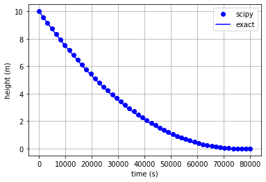
vars = change_input(res.x)
plt.plot(time, vars['h'], 'bo', label='scipy');
plt.plot( time, case1_exact(time),'b', label='exact')
plt.xlabel('time (s)')
plt.ylabel('height (m)')
plt.legend()
plt.grid();
Conclusion
In this post we have gone through the steps to implement the computational model of a lake using DAE approach. In the next post I will refactor a bit the interface to make it more modular and then proceed to the modelling of the reaches. I see you in the next post.
References
Himmelblau, D. M., & Riggs, J. B. (2006). Basic principles and calculations in chemical engineering. FT press.
Euan Russano, PhD
Tutor of Machine Learning, Artificial Intelligence, Statistics,…
I teach and train students, professionals and companies in Python, R, Machine Learning, Data Science and Statistics, among other subjects of interest.